Your Transformation Is Run by the Culture It Needs to Change
17 Nov 2026
Christian Kroschl · 2026 · exact date unconfirmed · English
The shop floor reports every completed operation, yet the planned lead time in the item master may have remained unchanged for years. This article traces the gap between feedback on orders and feedback on the assumptions behind them. Who owns the return path into planning parameters?
Complete PDF · 7 pages · 1.0 MB · Includes the full text and 3 full-size figures.
Archived local edition · The original publication date has not been confirmed.
Open the item master for a part you make. Look at the planned lead time. Now find out where that number came from and who changed it last.
Why the closed loop everyone cites has never closed around the fields it describes, why five separate traditions derived the return path and none of them wired it, and what a supply chain leader should ask a vendor before buying an agent.
In most plants the answer is that it arrived in the initial data load, was adjusted once during hypercare because orders were finishing late, and has not been touched since. The routing standard values behind it were set by a work study department that no longer exists. Meanwhile the shop floor has reported every operation completion for years.
That is the gap. Not a missing algorithm. A field that nobody writes to.
Closed loop MRP has been the standard term since the 1970s. Planning, execution, feedback, corrective action. Every planning system on the market implements it, and implements it correctly.
Look at what it actually closes. Confirmations return quantities and statuses. Order status drives receipt quantity and reservation quantity. The next regeneration converts the difference into exception messages: past due, reschedule in, reschedule out, cancel. That loop works. It has worked for fifty years.
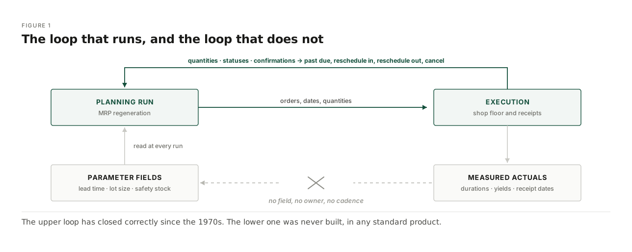
Now list what it does not touch. Planned lead time. Queue time. Lot size. Rounding value. Scrap and yield. Safety stock. Capacity assumption per work centre. Every one of those sits in the item master, the routing or the resource as a policy field. Every one of them is an input to the loop rather than an output of it.
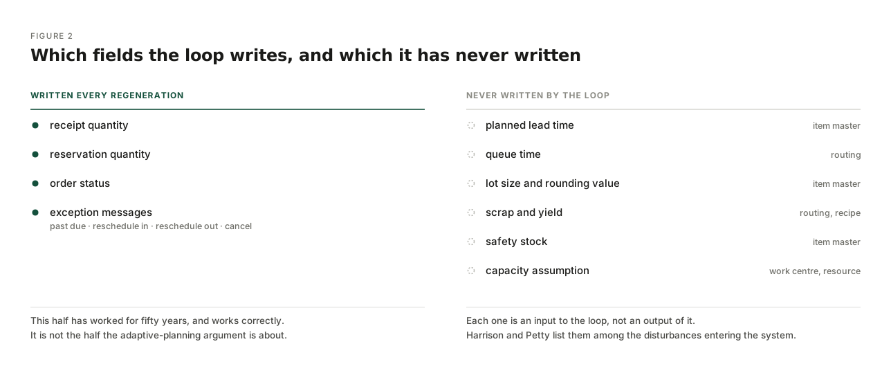
Harrison and Petty put this in writing in 2002. Their reference model lists planning changes such as lead times or lot sizes among the disturbances entering the system. Not among the results leaving it. The architecture was explicit about it, and the point passed without argument, because the order loop was doing its job and the plans looked plausible.
This is the part that should end the argument about whether adaptive planning is technically possible.
The German PPS school published the derivation in the nineties and Schuh carried it into a standard handbook in 2006. The funnel model relates input, WIP and output at a work centre. Mean range equals WIP divided by mean output rate. Vary WIP across observed operating states and you get the production operating curve, from which you read the planned lead time that belongs to a chosen operating point. In a case reported by Wiendahl and Nyhuis, a coating work centre ran at 26 standard hours of WIP, deep in the overload region. The curve said 5 hours was reachable without notable output loss. It was implemented, and they report a throughput time reduction at that work centre of roughly 80 percent.
The same school did it for stock. The storage operating curve sizes safety stock from the measured maxima of three plan deviations: receipt date deviation, demand rate during the replenishment lead time, and quantity under delivery. In the article spectrum they work through, target stock decomposed into 43 percent lot stock, 37 percent demand rate variation, 20 percent quantity deviation and under 1 percent delivery date deviation. Those figures come from their worked example rather than from a survey, and the point is not the split itself. It is that a planner can be told which cause to attack, and in what order.
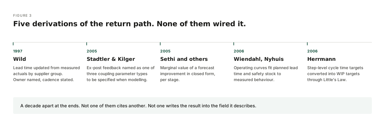
Wild did it from the inventory side in 1997. Safety stock equals the service factor times the measured deviation times the square root of the lead time. The MAD is smoothed every period. The lead time field is updated from measured actuals by exponentially weighted average, by supplier group. The forecast smoothing constant is reset by the tracking signal. He names the owner. He states the cadence: weekly or monthly, results inside three days of period end.
Herrmann's 2006 handbook carries a third version. SLIM-M at Samsung sets step level cycle time targets by allocating measured queue time to the constraint steps, then converts them into WIP targets through Little's Law.
Stadtler and Kilger, the canonical APS text, name the mechanism as a first class concept. Ex-post feedback is one of three coupling parameter types that have to be specified during model building, alongside instruction downward and reaction upward. The average realization of guidelines from the short term modules, they write, should be used for model adjustment in master planning.
Sethi and colleagues supplied the last piece in 2005, and it is the piece a business case needs: the marginal value of a forecast improvement in closed form, per stage, so the next unit of forecasting effort can be allocated on return rather than on conviction.
Five traditions. A decade apart at the ends. None of them cites another. All five derive the same thing. Not one of them writes the result into the field it describes.
The temptation is to call this an oversight. It was not, and the reason matters more than the observation.
Stadtler and Kilger leave the return path without a module. There is no box for parameter revision on their planning matrix. The loop is described as infrequent, and for structural change they advise manual adaptation of the model by an expert. That is a statement of need, not a mechanism.
Dickersbach shows what that means in a running system. Master data transfers one way, from the source of record into the planning system. Durations come from routing standard values through the scheduling formulas of the work centre at transfer time, then sit in the mode of the production data structure until someone changes the routing. Some objects carry no change pointer at all. A change to the work centre or to a phantom bill of material produces no notification, so a changed scheduling formula goes unnoticed. The alert monitor has six handling verbs: sort, confirm as checked, hide, show, freeze, branch. None of them changes a parameter. It notifies. It does not regulate. That was the design intent, and a defensible one: parameters are governed in the source of record, not regenerated by the planning system.
Hübner supplies the last part. In his specialty chemicals pilot the recipes pulled from ERP differed from the recipes actually used, in absolute quantities and in the proportions between raw materials. Yields for the same product differed significantly between sites. His comment is the one to keep: this appears to be the norm rather than a company specific exception.
So the return path is not missing because the loop was overlooked. It is missing because the measured object of record does not exist in the system that ought to hold it, and building it was never anyone's project.
Five things, and one of them is software.
A measured object of record. Actual operation duration against planned. Actual replenishment lead time against planned delivery time. Actual yield per site against recipe. Forecast by lag against actual, held at the aggregation the decision is taken on. That last one is a retention setting rather than a capability. In most installations the demand planning version is overwritten on release, so the history that would let you measure forecast quality by lag is not kept.
A named owner per parameter class. Wild put it on the inventory manager and defined the job as keeping the system parameters accurate rather than manually reinterpreting system output. That is the right job description, and it is not the one most planners have.
A cadence. None of the five sources except Wild states one.
A change threshold. This is the part that gets skipped. A closed loop without a dead band produces churn. Wild saw it as a practitioner: for A class items with unstable supply, stabilise the supplier rather than accelerate the parameter update, because each update changes the derived stock parameters and rewrites the open order book. Sethi derived the same result. Charge a fixed cost for amending an order and the optimal response to new information becomes a band, not a recomputation. Observe every period, act only when the position leaves the interval. The width of the band is a function of the cost of acting.
There is a second reason for the band that has nothing to do with cost. Sethi's field data shows that as the forecast horizon shortens, the variance of the forecast error falls and the variance of the forecast itself rises. The update series is more volatile than the plan it replaces, even while it is more accurate. If your order book is rewritten by every update, you are importing that volatility into your supply base.
A convergence check. Chandra and Grabis name the failure mode: if a parameter depends on a decision the next planning run may reverse, the loop oscillates and never settles. Updating a lead time from actuals produced under a sourcing decision that the next run reverses is exactly that case.
Two questions come before any of this.
Are standard values present on the routings. Without them WIP cannot be computed in standard hours and no operating curve can be fitted.
Are confirmations landing on the work centre that actually did the work. Schuh cites industrial studies reporting reject rates of 20 to 50 percent in confirmation data, with wrong work centre assignment the most frequent cause.
If either answer is no, the loop cannot be closed at any price. That is where the work starts.
The technology is not the constraint and has not been for a long time. APS, rule based sequencing, rhythm wheels, classical optimisation and demand driven methods all do what they claim. The derivations above were publishable, teachable and industrially proven before most current planning products shipped.
What was never built is the governed process that carries a measured number back into the field it describes, with an owner, a rhythm, and a rule for when not to act.
An agent that senses, decides and learns is being sold into that gap right now.
<callout icon="→" color="green_bg">
The question worth asking a vendor is not whether the model learns. It is this: which field does it write to, from which measurement, at what frequency, and who signs off the change.
If there is no answer, the loop is still open. It stays open no matter what runs on top of it.
</callout>
Two of the simulators on this site sit exactly on the fields this article is about. The Safety Stock Synthesizer shows which term is actually setting the buffer. The Lead Time Cascade shows what one lead time does to plan rigidity and to inventory at the same time. Both are the read side of the loop described here. Neither writes back either.
Christian Kroschl, August 2026. Figures are schematic. The case figures quoted are reported by the named authors, not collected here.
Questions about an article, a tool or a planning problem?